
Quick Navigation
Download Configuration Files
Statistical Downscaling Examples:
1. Delta Addition
2. Delta Correction
3. Quantile Mapping
4. Asynchronous Linear Regression
Acknowledgement
Statistical Downscaling using RCMES
Why do we need to downscale GCM outputs?
Global climate models (GCMs) cannot simulate climate at the local to regional scale.
RCMES utilizes the following statistical downscaling methods used in previous studies (e.g. Stoner et al. 2013).
- delta method
- bias correction - spatial disaggregation (BCSD)
- quantile mapping
- asynchronous regression approach
Advantages and Disadvantages of Statistical Downscaling
| Advantages | Disadvantages |
| Statistical Downscaling is relatively easy to produce. | There are assumptions of stationarity between the large and small scale dynamics when using statistical downscaling. |
| Impact-relevant variables not simulated by climate models can be downscaled using statistical downscaling. | Small scale dynamics and climate feedback are not reflected when statistical downscaling is used. |
| http://www.glisaclimate.org | |
This tutorial goes through four different methods of Statistical Downscaling. If you have not completed the Configuration File Training, you may want to do so now.
Download
Download and Install RCMES
If you have not installed RCMES, click here to do so now using either the Virtual Machine or Easy-OCW.
Download Model and Observation Datasets for Tutorial
CLICK HERE to download the data for this tutorial.
If you are using VM for this tutorial, place the Stat_dscale folder within your shared data folder that you set up during the VM Install. If you have restarted your machine since the last tutorial, you will need to remount your data folder.
If you are using Easy OCW for this tutorial, you will need to save your data to an appropriate place. It is recommended that you save your data in the /climate/RCMES/data folder.
Configuration File
The configuration file for this tutorial are found in the Statistical Downscaling directory within RCMES called statistical_downscaling.
In your terminal, navigate to the Statistical Downscaling directory.
cd /users/dlnash/rcmes/climate/examples/statistical_downscaling
Use the following command to list the files in the directory.
ls - l
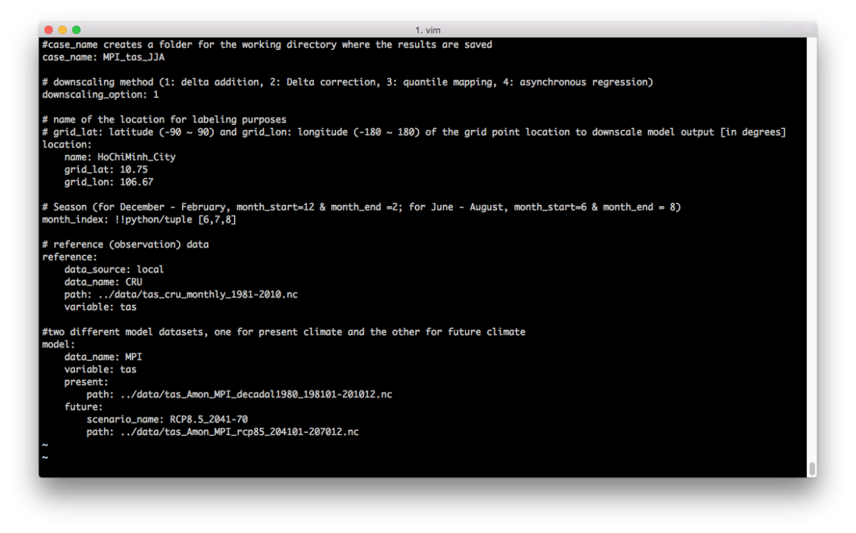
You should be able to see the run_statistical_downscaling.py and MPI_tas_JJA.yaml. Open the MPI_tas_JJA.yaml using the following command:
vim MPI_tas_JJA.yaml
This file functions similarly to the configuration files used for the 2013a and 2013b example pages. Examine the file (shown below) to see the breakdown.
Save any changes you have made to your configuration file and close the editor.
For these examples, all four methods of downscaling will be used for the city of Ho Chi Minh, Vietnam for the summer season. The results will be saved in the case_name folder specified in the MPI_tas_JJA.yaml and all figures are displayed below.
Run Statistical Downscaling Examples
Method 1: Statistical Downscaling using Delta Addition
The difference between present and future simulations are added to the present observation - See Plot 1 below.
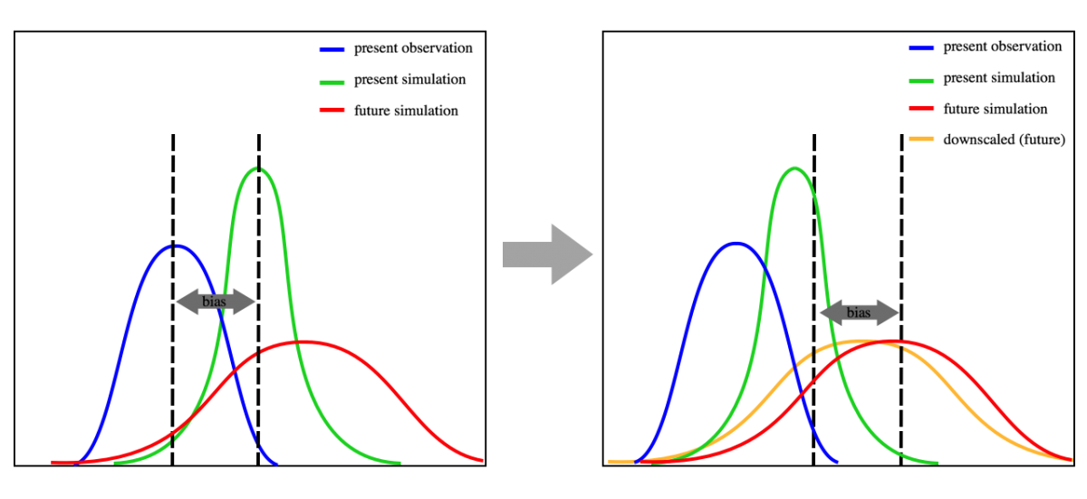
First, the mean difference between present simulation (green) and future simulation (red) is calculated. And the calculated difference is added to the present observation (blue) to make a downscaled future prediction. In this method, only the change in mean values in simulations is considered in the future projection.
 |
| (Plot 1) (downscaled future) = (present observation) + (mean difference between present simulation and future simulation) |
Compile and run the statistical downscaling.
python run_statistical_downscaling.py MPI_tas_JJA.yaml
In the 'case_name' folder specified in the configuration file, figure results and an excel spreadsheet file are found.
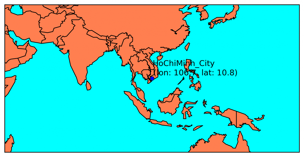 |
| (Fig. 1a) This result is a map of the indicated location with a marker, Ho Chi Minh, Vietnam. |
| Original Distribution | Downscaled Distribution using Delta Addition |
 |
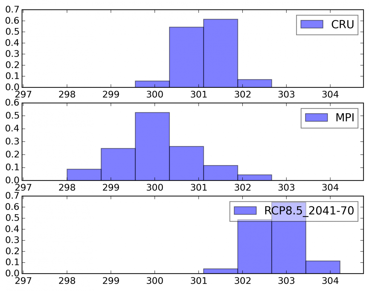 |
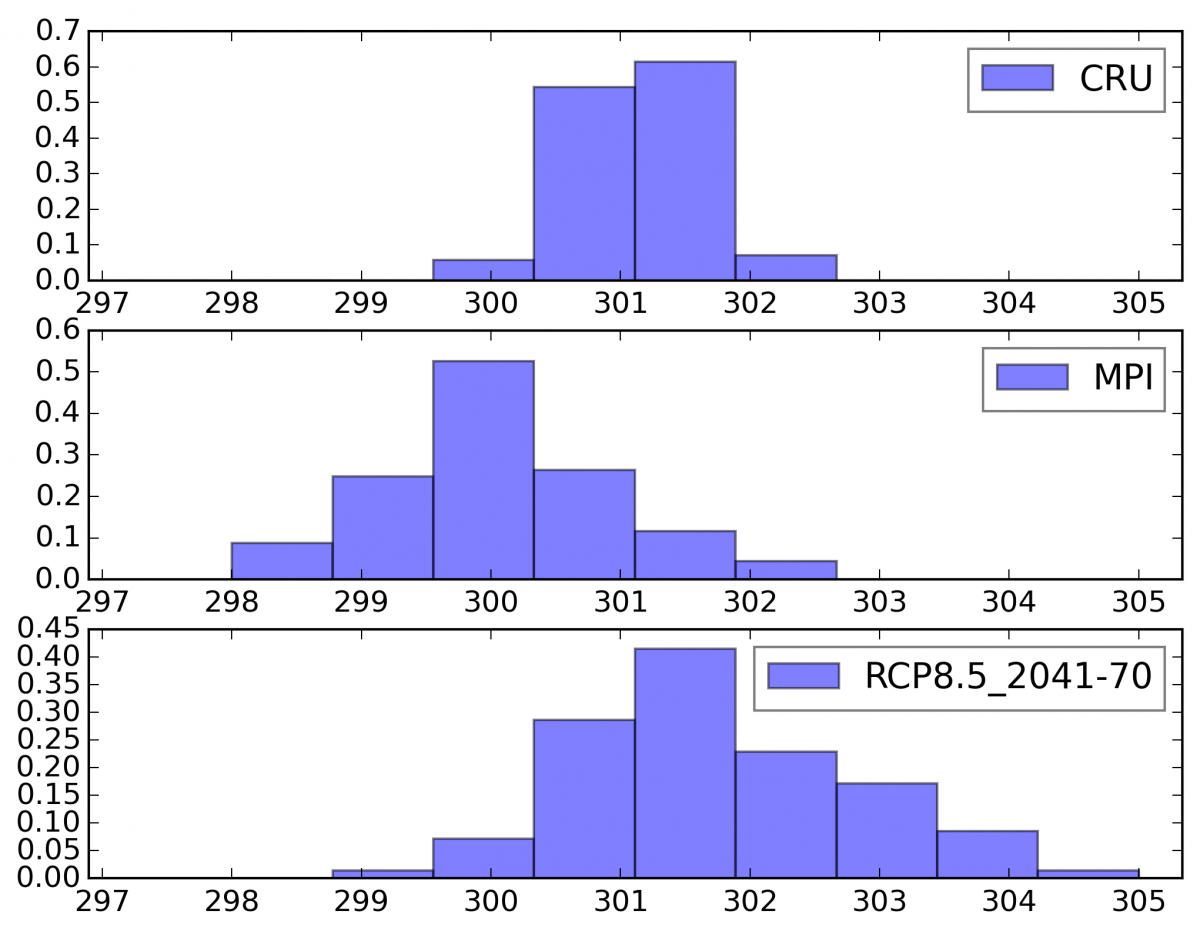
| (Fig 1b) This figure shows the histogram of the original temperature distribution before the data from June through August is downscaled. | (Fig 1c) This figure shows the downscaled data distribution using the Delta Addition Method from June through August for Ho Chi Minh, Vietnam. |
The excel spreadsheet includes the downscaling location, months indicated, observational data, model data, and downscaled data.
Method 2: Statistical Downscaling using Delta Correction
Only mean biases of models are corrected.
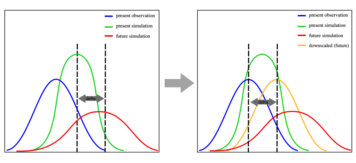
In this method, the mean bias of present simulation (green) from present observation (blue) is calculated and added to the future simulation [left diagram]. So the downscaled future simulation (yellow) has zero mean bias to the present observation [right diagram].
 |
| (Plot 2) (downscaled future) = (future simulation) + (mean bias of present simulation from present observation) |
Edit the MPI_tas_JJA.yaml to change the downscaling method to 2 (delta correction). Compile and run the statistical downscaling.
python run_statistical_downscaling.py MPI_tas_JJA.yaml
| Original Distribution | Downscaled Distribution using Delta Correction |
|
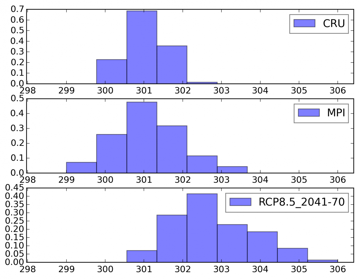 |
| (Fig 2a) This figure shows the histogram of the original temperature distribution before the data from June through August is downscaled. | (Fig 2b) This figure shows the downscaled data distribution using the Delta Correction Method from June through August for Ho Chi Minh, Vietnam. |
The excel spreadsheet includes the downscaling location, months indicated, observational data, model data, and downscaled data.
Note: The spreadsheet should add a new sheet with the different method information.
Method 3: Statistical Downscaling using Quantile Mapping
In this method, biases are calculated for each percentile in the cumulative distribution function from present simulation (blue). Then the calculated biases are added to the future simulation to correct the biases of each percentile.
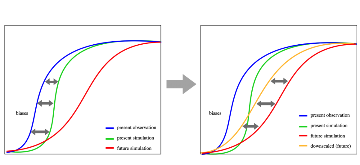 |
| (Plot 3) (downscaled future) = (calculated bias for cumulative distribution functions from present observation to present simulation) + (future simulation) |
Edit the MPI_tas_JJA.yaml to change the downscaling method to 3 (quantile mapping). Compile and run the statistical downscaling.
python run_statistical_downscaling.py MPI_tas_JJA.yaml
| Original Distribution | Downscaled Distribution using Quantile Mapping |
|
 |
| (Fig 3a) This figure shows the histogram of the original temperature distribution before the data from June through August is downscaled. | (Fig 3b) This figure shows the downscaled data distribution using the Quantile Mapping Method from June through August for Ho Chi Minh, Vietnam. |
The excel spreadsheet includes the downscaling location, months indicated, observational data, model data, and downscaled data.
Note: The spreadsheet should add a new sheet with the different method information.
Method 4: Statistical Downscaling using Asynchronous Linear Regression
If we plot a scatter plot of observed data (x-axis) versus simulated data by CMIP5 (y-axis), it is hard to expect a statistically significant relationship as shown in the left side of Plot 4 (below).
This is because the GCM-simulated climate in specific time is unrelated to the real climate at the same time. However, when the time series from observation and a model are sorted in ascending order, the linear relationship can be seen as in the right side of Plot 4.
The asynchronous linear regression finds the linear relationship between the sorted observation and model time series.
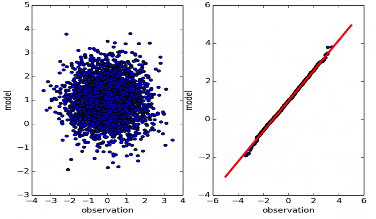 |
| (Plot 4) The plot on the left shows the scatter plot of the original model and observation data. The figure on the right shows the linear relationship between observation and present simulation after sorting them in ascending order. |
Edit the MPI_tas_JJA.yaml to change the downscaling method to 4 (asynchronous regression). Compile and run the statistical downscaling.
python run_statistical_downscaling.py MPI_tas_JJA.yaml
| Original Distribution | Downscaled Distribution using Asynchronous Linear Regression |
|
 |
| (Fig 4a) This figure shows the histogram of the original temperature distribution before the data from June through August is downscaled. | (Fig 4b) This figure shows the downscaled data distribution using the Asynchronous Linear Regression Method from June through August for Ho Chi Minh, Vietnam. |
The excel spreadsheet includes the downscaling location, months indicated, observational data, model data, and downscaled data.
Note: The spreadsheet should add a new sheet with the different method information.
Acknowledgement
We would like to thank the APEC Climate Center (APCC) for creating the opportunity for the collaboration between JPL/NASA and the Vietnam Institute of Meteorology, Hydrology and Climate Change (IMHEM). This collaboration enabled the use of RCMES in statistical downscaling of climate change over Vietnam, which has been posted as an exemplary training on the RCMES website.