The Regional Climate Model Evaluation System (RCMES) is a comprehensive suite of software resources to standardize and streamline the process of interacting with observational data and climate model output to conduct regional climate model evaluations. The system and workflow are schematically illustrated in Fig. 1. On the left are provisions for reading in observations from a number of sources, including from obs4MIPs and ana4MIPs, datasets that reside on the user's local disk that were obtained from other data centers, and for a few cases observation datasets included in the RCMES distribution. On the right is the typical workflow that includes ingesting model data, typically a regridding step to place the model and observations on the same grid for analysis, and then steps to perform analysis and visualization. RCMES software is powered by the Open Climate Workbench (OCW) that includes a library for common model evaluation tasks (e.g.: area averaging, regridding, bias calculation) as well as a set of user-friendly interfaces for quickly configuring a large-scale regional model evaluation task. These include the Command Line Interface (CLI) and Configuration Files (CF) briefly described below.
RCMES is packaged as a Virtual Machine image that contains all of the software, dependencies, libraries, configuration files, sample observation and model datasets, etc. needed to quickly get up and running with a model evaluation experiment. The virtual machine packaging dramatically reduces the time required to obtain the necessary environment for experimenting with RCMES. RCMES supports a wide variety of use cases, from simple non-connected tasks like performing re-gridding of model and observational data, to a complete model evaluation workflow from configuration to output plots. To download RCMES, follow the steps on Download RCMES.
Figure 2 illustrates the pathway for Getting Started using RCMES via the Tutorials Overview. The first step is to learn about RCMES basics through the simple Command Line Interface (CLI). The CLI is intended primarily only for training, not to support general model evaluation tasks. By following the CLI training material, a user can learn the basic workflow associated with RCMES. This typically takes the form of inputting model datasets, observations, specifying gridding options and analysis and associated plotting function. Once the CLI is understood, the next level of detail and capability is provided by RCMES Configuration Files (CFs). These are configurable files that provide input to the RCMES workflow and processing engine and allow for basic and more advanced model evaluation capabilities. The Configuration File training material illustrates the use of these files in producing the plots/diagrams in previously published RCMES supported peer-reviewed journal articles (e.g. Kim et al. 2013, Clim. Dyn). For more advanced model evaluation considerations within the context of RCMES, the user is referred to the material on the Open Climate Workbench (OCW), and encouraged to utilize the underlying software directly and share any additions or enhancements via the open source protocol of OCW.
A typical RCMES workflow consists of the following steps (a simple python script):
The OCW (python) library provides a set of functions implementing each of these steps (e.g. local.load_file, temporal_regrid, spatial_regrid, etc.). See the tutorials and example scripts for how to use them.
RCMES provides convenient access to multiple sources of data:
The OCW readers can ingest data on regular grids (lat/lon/alt coordinates are vectors) or high-resolution irregular grids (lat/lon coordinates are a 2-dimensional mesh). For netCDF files that satisfy the Climate Forecast (CF) metadata conventions, attributes and metadata are automatically recognized and extracted (offset, scale, units, etc.). Adding another reader for a specific file format can usually be easily done in python.
The OCW library provides a set of functions to subset and interpolate data in space and time. Global grids can be subsetted onto a region and then spatially interpolated onto a common spatial grid using bi-linear interpolation or other interpolation schemes. Time-series can be interpolated to weekly, monthly, or annual boundaries for comparisons. [more here]
It is easy to add metrics to the OCW library using the matrix algorithms available in the python numpy and scipy libraries. OCW currently evaluates a full set of statistical metrics commonly used in model evaluation, including:
OCW also contains a sub-region capability. Each metric can be computed on the entire study region and on a set of sub-regions. For examples of this usage, see the tutorial on regional (“downscaled”) model evaluation for CORDEX (Coordinated Regional Climate Downscaling Experiment) Africa.
Computed metrics can be downloaded or visualized in standard plots. For example, the Standard Deviation Ratio and Pattern Correlation can be combined into a Taylor diagram. Some examples of analysis plots from a CORDEX Africa analysis appear below (see the tutorials to learn how to reproduce them).
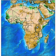
Basemap with marked sub-regions
This generic map with sub-regions always plots with metrics that have sub-regions set to True.
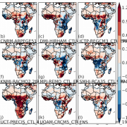
Bias comparison for multiple models
Metric Name: Map_plot_bias_of_multiyear_climatology
This metric produces a bias plot of the observation against individual models.
The annual mean of the chosen variable is plotted over the spatial boundaries for each model as well as for the observation data set.
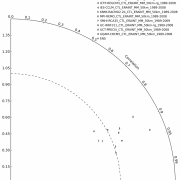
Taylor Diagram
Metric Name: Taylor_diagram_spatial_pattern_of_multiyear_climatology
This metric produces a Taylor Diagram of spatial pattern correlations and standardized deviations with respect to the observation.
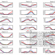
Monthly model comparison for sub-regions
Metric Name: Timeseries_plot_subregion_annual_cycle
This metric produces a time series plot for the defined sub-regions. Annual monthly means for the variable defined are plotted for each model and the observation data sets.
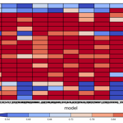
Sub-region correlations for multiple models
Metric Name: Portrait_diagram_subregion_annual_cycle
This metric produces four portrait diagrams for all defined sub-regions.
For each sub-region and model defined, the bias, standard deviation, correlation, and RMSE are shown.